Video and reference

Please refer to this paper when you cite any work from this blog:
Semi-autonomous navigation for robot assisted tele-echography using generalized shape models and co-registered RGB-D cameras
Lin Zhang and Su-Lin Lee and Guang-Zhong Yang and Mylonas, G.P.
Intelligent Robots and Systems (IROS 2014), 2014 IEEE/RSJ International Conference on

Experiment on effect of differently cropped shape on SSM

In order to achieve better validation result, I am trying to use the shape models that were cropped differently according to target object.
As the back of subject cannot been seen by both Kinects and the plastic torso is rigid and not as same as human torso, I tried to use shapes whose back have been cropped (shown in Figure 1).

Figure 1 Torso shape model (no head, legs, arms and back)

For real human subject, since the head and arms are required (no head nor arms for the plastic torso), I remain the head and part of arm for shape model training (shown in Figure 2).

Figure 2 Torso shape model (no legs, part arms and no back)

Colour Point Cloud detection and extraction based on HSV colour space

In order to register the Kinects with KUKA robot which is fixed on a optical table, I use three color markers whose position is known within KUKA coordinate system.
Here is a snapshot of the markers:

Figure 1 Three colour markers with three different colours (R, G, B)

As shown in the Figure 1, three markers are painted as red, green and blue respectively. These three markers are read as RGB point cloud from the Kinect after combining depth image with colour image. However, similar colours describing by RGB components are not easy to distinguish with each other if environment illumination is variant from time to time, therefore, difficult to choose thresholds of colour components for point cloud filtering.

To address above weakness, instead of using RGB colour space, we can use HSV (Hue, Saturation and Value) space for colour representation. The following figure shows that how value of the hue, saturation and value components can be changed.
Hue: 0 - 360 (°)
Saturation: 0 - 100 (%)
Value: 0 - 100 (%)

Figure 2 HSV colour space can be visualised as a single cone [1]

For my markers, I used following conditions to extract them out:
RED: 
if (HSV_map_->points[i].s <= 0.2 || HSV_map_->points[i].v <= 0.2)
// Not target colour
if (HSV_map_->points[i].s <= 0.4 && HSV_map_->points[i].v <= 0.4)
// Not target colour
if (HSV_map_->points[i].h >= 350 || HSV_map_->points[i].h < 10)
// Can be target colour

GREEN:
if (HSV_map_->points[i].s <= 0.3 || HSV_map_->points[i].v <= 0.3)
// Not target colour
if (HSV_map_->points[i].h >= 100 && HSV_map_->points[i].h < 140)
// Can be target colour

BLUE:
if (HSV_map_->points[i].s <= 0.3 || HSV_map_->points[i].v <= 0.3)
// Not target colour
if (HSV_map_->points[i].h >= 220 && HSV_map_->points[i].h < 260)
// Can be target colour

After the potential target colour points are extracted, we need to filter out the outliers caused by noises. Here we need to have an assumption that the marker is the largest objects (most number of points) with that specific colour within field of view. Hence, it is able to use Euclidean Cluster Extraction algorithm implemented in PCL (link) to get the largest cluster which hopefully is our marker. Since the marker has circular shape, mean value of the extracted points can be treated as centre of the marker.

Based on the calculation so far, it is able to get position three points in 3D space in both coordinates. The transformation (only rotation + rotation) between two coordinates is able to calculated using PCL function pcl::registration::TransformationEstimationSVD::estimateRigidTransformation (link).


Results:

Experiment 1: Three markers are placed on a flat table. First coordinate is same as Kinect coordinate. The origin of second coordinate is defined as centre of the red marker while red-green is x-axis and red-blue is y axis. Since right hand coordinate was used, the z axis of the second coordinate is upward out of table. The lengths of red-green line and red-blue line are both 30 cm measured by ruler.

Figure 3 Result of experiment 1

From the Figure 3, we can see that the Kinect coordinate was almost perfectly aligned with the coordinate defined by ourself.

Experiment 2: In this experiment, I tried to align two Kinects using this method. The process is basically identical except that the extra Kinect introduces one more time colour detection and extraction process.
From the Figure 4, we can see that the result is quite good as the top side of the box is aligned without any visible error.

Figure 4 Animation that shows good alignment of point clouds from two Kinects

Reference:
[1] Microsoft Dev Centre - Color : link

Circular trajectory based on Start and End point

By knowing start and end point of a trajectory, we want to create a circular trajectory which can avoid body and provide smooth path for robot navigation.


Middle Point Generation:

A circle is unique if and only if three points are known, therefore, we need to calculate the middle point between the start and end point. As shown in Figure 1, we have two points P1 and P4 on a plane which is assumed to be parallel to table. In order to find the middle point, we artificially create two points P2 and P3 which have same x-axis offset to P4 and P1 respectively. Next, we connect P1 with P2 and P4 with P3 by which two lines are intersected. From the intersection point, we can estimate its normal and therefore create our middle point by extending the point at normal direction. Note that the normal must be upward so the trajectory will cross over body rather then go under table.

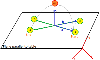
Figure 1 schematic of middle point generation based on two end points

Circle calculation (centre and radius):
Let's label the start, middle and end point to 0, 1 and 2. Here is snippet for the circle calculation:

 /*
  Circle calculation algorithm refer to:
  Implementation of arc interpolation in a robot by using three arbitrary points (Chinese), Ye Bosheng, 2007
 */
 float a00, a01, a02, a10, a11, a12, a20, a21, a22, b0, b1, b2;

 // Matrix A (3x3)
 a00 = 2 * (Cstart_[0] - Cmiddle_[0]); // 2 * (X0 - X1)
 a01 = 2 * (Cstart_[1] - Cmiddle_[1]); // 2 * (Y0 - Y1)
 a02 = 2 * (Cstart_[2] - Cmiddle_[2]); // 2 * (Z0 - Z1)

 a10 = 2 * (Cmiddle_[0] - Cend_[0]);  // 2 * (X1 - X2)
 a11 = 2 * (Cmiddle_[1] - Cend_[1]);  // 2 * (Y1 - Y2)
 a12 = 2 * (Cmiddle_[2] - Cend_[2]);  // 2 * (Z1 - Z2)
 
 a20 = a02 * (a02 * a11 - a01 * a12) / 8;
 a21 = a02 * (a00 * a12 - a02 * a10) / 8;
 a22 = - (a00 * (a02 * a11 - a01 * a12) + a01 * (a00 * a12 - a02 * a10)) / 8;

 // Matrix B (3x1)
 // b0 = (X0^2 + Y0^2 + Z0^2) - (X1^2 + Y1^2 + Z1^2)
 b0 = (Cstart_[0]*Cstart_[0] + Cstart_[1]*Cstart_[1] + Cstart_[2]*Cstart_[2])
  - (Cmiddle_[0]*Cmiddle_[0] + Cmiddle_[1]*Cmiddle_[1] + Cmiddle_[2]*Cmiddle_[2]);

 // b1 = (X1^2 + Y1^2 + Z1^2) - (X2^2 + Y2^2 + Z2^2)
 b1 = (Cmiddle_[0]*Cmiddle_[0] + Cmiddle_[1]*Cmiddle_[1] + Cmiddle_[2]*Cmiddle_[2])
  - (Cend_[0]*Cend_[0] + Cend_[1]*Cend_[1] + Cend_[2]*Cend_[2]);

 // b2 = a20*X0 + a21*Y0 + a22*Z0
 b2 = a20 * Cstart_[0] + a21 * Cstart_[1] + a22 * Cstart_[2];

 Eigen::Matrix3f A;
 Eigen::Vector3f B;

 A << a00, a01, a02, 
   a10, a11, a12,
   a20, a21, a22; 
 B << b0, b1, b2;

 /* 
  Centre of circle [Xc Yc Zc] can be calculated as
  A * [Xc Yc Zc]' = B;
  For Eigen library solving Ax = b, refer to:
  http://eigen.tuxfamily.org/dox/TutorialLinearAlgebra.html
 */
 Ccentre_= A.colPivHouseholderQr().solve(B);
 
 /*
  Radius of circle can be calculated as:
  R = [(X0 - Xc)^2 + (Y0 - Yc)^2 + (Z0 - Zc)^2]^0.5
 */
 float temp_equa;
 temp_equa = (Cstart_[0] - Ccentre_[0]) * (Cstart_[0] - Ccentre_[0]);
 temp_equa += (Cstart_[1] - Ccentre_[1]) * (Cstart_[1] - Ccentre_[1]);
 temp_equa += (Cstart_[2] - Ccentre_[2]) * (Cstart_[2] - Ccentre_[2]);
 radius_ = sqrt(temp_equa);

Trajectory interpolation:
Here is the snippet for determining central angle:

 /*
  normal of circle plane
  u = (Y1 - Y0)(Z2 - Z1) - (Z1 - Z0)(Y2 - Y1)
  v = (Z1 - Z0)(X2 - X1) - (X1 - X0)(Z2 - Z1)
  w = (X1 - X0)(Y2 - Y1) - (Y1 - Y0)(X2 - X1)
 */
 Cnu_ = (Cmiddle_[1] - Cstart_[1]) * (Cend_[2] - Cmiddle_[2]) - (Cmiddle_[2] - Cstart_[2]) * (Cend_[1] - Cmiddle_[1]);
 Cnv_ = (Cmiddle_[2] - Cstart_[2]) * (Cend_[0] - Cmiddle_[0]) - (Cmiddle_[0] - Cstart_[0]) * (Cend_[2] - Cmiddle_[2]);
 Cnw_ = (Cmiddle_[0] - Cstart_[0]) * (Cend_[1] - Cmiddle_[1]) - (Cmiddle_[1] - Cstart_[1]) * (Cend_[0] - Cmiddle_[0]);

 // normal vector to determine central angle
 float u1, v1, w1;
 u1 = (Cstart_[1] - Ccentre_[1]) * (Cend_[2] - Cstart_[2]) - (Cstart_[2] - Ccentre_[2]) * (Cend_[1] - Cstart_[1]);
 v1 = (Cstart_[2] - Ccentre_[2]) * (Cend_[0] - Cstart_[0]) - (Cstart_[0] - Ccentre_[0]) * (Cend_[2] - Cstart_[2]);
 w1 = (Cstart_[0] - Ccentre_[0]) * (Cend_[1] - Cstart_[1]) - (Cstart_[1] - Ccentre_[1]) * (Cend_[0] - Cstart_[0]);

 float H, temp;
 H = Cnu_ * u1 + Cnv_ * v1 + Cnw_ * w1;
 temp = (Cend_[0] - Cstart_[0]) * (Cend_[0] - Cstart_[0]) + 
   (Cend_[1] - Cstart_[1]) * (Cend_[1] - Cstart_[1]) +
   (Cend_[2] - Cstart_[2]) * (Cend_[2] - Cstart_[2]);
 if (H >= 0) // theta <= PI
 {
  Ctheta = 2 * asin(sqrt(temp) / (2 * radius_));
 } 
 else  // theta > PI
 {
  Ctheta = 2 * M_PI - 2 * asin(sqrt(temp) / (2 * radius_));
 }

Here is the snippet for calculation of number of points to be interpolated:

int CircleGenerator::CalcNbOfPts(const float &step)
{
 float temp;
 temp = 1 + (step / radius_) * (step / radius_);
 paramG_ = 1 / sqrt(temp);

 temp = Cnu_*Cnu_ + Cnv_*Cnv_ + Cnw_*Cnw_;
 paramE_ = step / (radius_ * sqrt(temp));

 float sigma;
 sigma = step / radius_;

 int N;
 N = (int)(Ctheta / sigma) + 1;

 return (N);
}

Here is the snippet for calculating next point in the trajectory:

 traj->push_back(vector2pcl(circle_->Cstart_));
 for (int i = 1; i < numOfPt; i++)
 {
  /*
   Equation 8:
   mi = v(Zi - Zc) - w(Yi - Yc)
   ni = w(Xi - Xc) - u(Zi - Zc)
   li = u(Yi - Yc) - v(Xi - Xc)
  */
  if (i == 1)
  {
   pre = circle_->Cstart_;
  }
  float mi, ni, li;
  mi = circle_->Cnv_ * (pre[2] - circle_->Ccentre_[2]) - circle_->Cnw_ * (pre[1] - circle_->Ccentre_[1]);
  ni = circle_->Cnw_ * (pre[0] - circle_->Ccentre_[0]) - circle_->Cnu_ * (pre[2] - circle_->Ccentre_[2]);
  li = circle_->Cnu_ * (pre[1] - circle_->Ccentre_[1]) - circle_->Cnv_ * (pre[0] - circle_->Ccentre_[0]);
  
  /*
   X(i+1) = Xc + G * (X(i) + E*mi - Xc)
   Y(i+1) = Yc + G * (Y(i) + E*ni - Yc)
   Z(i+1) = Zc + G * (Z(i) + E*li - Zc)
  */
  curr[0] = circle_->Ccentre_[0] + circle_->paramG_ * (pre[0] + circle_->paramE_ * mi - circle_->Ccentre_[0]);
  curr[1] = circle_->Ccentre_[1] + circle_->paramG_ * (pre[1] + circle_->paramE_ * ni - circle_->Ccentre_[1]);
  curr[2] = circle_->Ccentre_[2] + circle_->paramG_ * (pre[2] + circle_->paramE_ * li - circle_->Ccentre_[2]);
  traj->push_back(vector2pcl(curr));
  pre = curr;
 }
 traj->push_back(vector2pcl(circle_->Cend_));

Point cloud normal estimation and Correspondence based on Normal shooting

Souce cloud: shape model

Target cloud: point cloud from Kinect

Normal cloud: a cloud of normal for shape model cloud

Step 1: Normal estimation based on point cloud itself

Step 2: Figure out the normal direction based on the view port position

Step 3: Find the correspondence in target cloud for each point in source cloud (shape model)

Results:

Figure 1 Red points: shape model cloud; Blue line: normal starts from point; colorful point: cloud from Kinect

Figure 2 Side view of Figure 1.

Figure 3 Top view of Figure 1.

Figure 4 Green points are the correspondences obtained from normal shooting

Calculating Euler angles from a rotation matrix

For rotation with inverse order Rzxy, refer to here.

Finding transformation between corresponding 3D points

With the shape model registered with point cloud, we need to align it with the mean model so that they are in same reference frame and comparable.
The transformation between shape model and mean model includes translation, scaling and rotation.

Translation:
In order to make two shape comparable, I translate both registered shape model and mean model to origin.

Scaling:
A simple way is to normalize the shape itself which results in a scaled shape of size 1. The size of shape is calculated by Opencv cv::norm() which computes an absolute array norm based on following equation.

In my program I use NORM_L2.

Rotation:
Now the registered shape model and the mean shape are almost aligned except the rotation. As the correspondences between two shape are known information, the rotation matrix can be solved using SVD (singular vector decomposition) which is introduced here.
Firstly, we need to decompose matrix H which is:

As the centroid of two shape has been subtracted already in the translation part, we can just put PA and PB as our two shapes. Next, the SVD of H is:

Finally, the rotation matrix from shape A to shape B can be calculated using U and V:

If we want to get rotation from shape B to A, just alter the equation to PB*PA instead of PA*PB.


Reference:
[1] Finding optimal rotation and translation between corresponding 3D points
[2] OpenCV document

Registration using Normal Distribution Transformation

In this post, I am going to experiment the PCL Normal Distribution Transformation (NDT) algorithm for registration of two clouds.

Experiment description:

Two Kinects are oppositely located and both facing to a box of size ~18x40cm on a table. One Kinect is called target and the other is called source. Therefore, our aim is to register source cloud with target cloud, or in other word find a transformation that best align source cloud and target cloud.
Both source and target clouds have been cropped based on region of interest for faster processing and fewer background noise. In addition, source cloud (coloured with green) has been down-sampled to 1/10 of its original density.

As mentioned at PCL official tutorial (link), these parameters are set according to different application:

The Transformation Epsilon(TE) parameter defines minimum, allowable, incremental change of the transformation vector, [x, y, z, roll, pitch, yaw] in meters and radians respectively. Once the incremental change dips below this threshold, the alignment terminates.

The Step Size(SS) parameter defines the maximum step length allowed by the More-Thuente line search. This line search algorithm determines the best step length below this maximum value, shrinking the step length as you near the optimal solution. Larger maximum step lengths will be able to clear greater distances in fewer iterations but run the risk of overshooting and ending up in an undesirable local minimum.

The Resolution parameter(RP) defines the voxel resolution of the internal NDT grid structure. This structure is easily searchable and each voxel contain the statistical data, mean, covariance, etc., associated with the points it contains.

I've adjusted these parameters individually and cross compared the results of registration.

TE: 0.01, SS:0.01, RP:0.1

TE: 0.01, SS:0.01, RP:0.1

TE: 0.01, SS:0.01, RP:0.2

TE: 0.01, SS:0.01, RP:0.2

TE: 0.01, SS:0.01, RP:0.3

TE: 0.01, SS:0.01, RP:0.3

TE: 0.01, SS:0.05, RP:0.1

TE: 0.01, SS:0.05, RP:0.1

TE: 0.01, SS:0.05, RP:0.3

TE: 0.01, SS:0.05, RP:0.3

From above results we can conclude:
1) If the clouds were jointing together rather than aligning, we can increase the RP in order to include more points for each voxel structure.
2) For large SS parameter, the registration converge faster while small SS parameter gives finer alignment.

At the end of experiment, I found that the algorithm is more robust to regular object in the scene. Since the above experiment all includes my head during registration. If I let myself out of the scene, the registration can be done much better and faster for reasonable parameters. Here is the result without my head in the scene:

TE: 0.01, SS:0.01, RP:0.2

TE: 0.01, SS:0.01, RP:0.2

Reference
[1] Merten, H. (Ed.). (2008). The Three-Dimensional Normal-Distributions Transform. threshold, 10, 3.

VOSM installation in VS2010 NO CMAKE

This post is just for own reference only.

Step 1: Download vosm for windows (link)

Step 2: Unzip

Step 3: Open vosm.sln

Step 4: For all projects (comalgs; common; cvcommon; ensembletraining; featureextraction; integraltransform; smbuilding; smfitting; test_ensembletraining; test_featureextraction; test_integraltransform; test_smbuilding; test_smfitting)
configure boost and opencv lib and include directory for both DEBUG and RELEASE mode. Keep additional DIR under【C/C++】-【General】-【Additional Include Directories】in RELEASE mode same as DEBUG mode.

Step 5: For project comalgs; common; cvcommon; ensembletraining; featureextraction; integraltransform; smbuilding; smfitting, change configuration type under 【Project Defaults】-【Configuration Type】-【Additional Dependencies】to Static library (.lib)

Step 6: For projects test_ensembletraining; test_featureextraction; test_integraltransform; test_smbuilding; test_smfitting, add .lib file name of opencv and boost library correctly【Linker】-【Input】-【Additional Dependencies】in both DEBUG and RELEASE mode.
Boost Debug:
libboost_regex-vc100-mt-gd-1_49.lib
libboost_filesystem-vc100-mt-gd-1_49.lib
libboost_system-vc100-mt-gd-1_49.lib
Boost Release:
libboost_regex-vc100-mt-1_49.lib
libboost_filesystem-vc100-mt-1_49.lib
libboost_system-vc100-mt-1_49.lib

Step 7: Under【Linker】-【General】-【Additional Library Directories】, input ../../Debug and ../../Release for DEBUG and RELEASE mode respectively.

Step 8: Compile all projects (modules then tests) in both Debug and Release mode.

Solve linear least-square problem using OpenCV (Reference)

C++: bool solve(InputArray src1, InputArray src2, OutputArray dst, int flags=DECOMP_LU)

Parameters:

• src1 – input matrix on the left-hand side of the system.

• src2 – input matrix on the right-hand side of the system.

• dst – output solution.

• flags –

solution (matrix inversion) method.

• DECOMP_LU Gaussian elimination with optimal pivot element chosen.

• DECOMP_CHOLESKY Cholesky  factorization; the matrix src1 must be symmetrical and positively defined.

• DECOMP_EIG eigenvalue decomposition; the matrix src1 must be symmetrical.

• DECOMP_SVD singular value decomposition (SVD) method; the system can be over-defined and/or the matrixsrc1 can be singular.

• DECOMP_QR QR factorization; the system can be over-defined and/or the matrix src1 can be singular.

• DECOMP_NORMAL while all the previous flags are mutually exclusive, this flag can be used together with any of the previous; it means that the normal equations  are solved instead of the original system  .

The function solve solves a linear system or least-squares problem (the latter is possible with SVD or QR methods, or by specifying the flag DECOMP_NORMAL ):

If DECOMP_LU or DECOMP_CHOLESKY method is used, the function returns 1 if src1 (or  ) is non-singular. Otherwise, it returns 0. In the latter case, dst is not valid. Other methods find a pseudo-solution in case of a singular left-hand side part.

In my case, I have equation min|| P*b - (Xnew - Xm) || to solve. P is mxp eigenvector, Xnew is the target shape, Xm is the mean shape in trained model, b is the shape parameter vector we want to get. m is number of attributes (number of point * 3), p is the number of reduced eigenvalue.

Reference: http://docs.opencv.org/modules/core/doc/operations_on_arrays.html#solve

Octree based point cloud stream compression in PCL

The point cloud produced from Kinect-like sensor is dense and updated at real-time frame rate (30 Hz). At usual case, 240k ~ 270k points are generated per second per Kinect depend on complexity of scene. As the dynamic point clouds are sampled at 30 Hz, it contains a total of about 7.5 million points per second. Since two Kinects have been used in this project, double of the point cloud is required to transmit.
The Point Cloud Library (PCL) has implemented an octree based compression class which enables both spacial and temporal compression at the same time. The full framework of the algorithm is introduced in [1].

Spacial compression:
The point cloud is decomposed into nodes by employing an octree structure which can be briefly illustrated as Figure 1. When constructing the octree, every node occupied by point(s) is set to non-empty (filled black in the figure). For each node contains point(s), we can further subdivide into 8 octants until the number of level or size of node reaches our predefined threshold. The child node configuration can be efficiently represented in a single byte (8-bit for 8 octants). Therefore, the whole octree structure is encoded into a stream, and the size of the stream equals to the number of branch nodes (unit is byte).

Figure 1 Schematic overview of the octree data structure and its serialization [1].

Temporal compression:
Since changes in the point cloud of the captured scene often occur only partially in confined areas, the correlation between currently sampled points and previously encoded point cloud can be exploited to improve compression performance. In [1] authors proposed a double-buffering octree method to solve the problem. Instead of eight child pointers to child nodes, the double-buffering use an additional set of eight child pointers to every branch. As shown in Figure 2, let's call them buffer A and B. Two buffers are alternatively assigned to every new captured point cloud. It is pointed out in the paper that the current point cloud in one octree structure allows us to spatially match, reference and analyse the structural changes within consecutive octree structure [1].

Figure 2 Illustration of differential encoding technique when using double-buffering octree [1].

In order to obtain and output the structural changes for every branch of two consecutive point clouds, the authors applied an exclusive disjunction operation (XOR) on the two bytes representing the node configuration for that branch over the whole octree structure.

Compression architecture:
In addition to the spacial and temporal encoded information as introduced above, for more precise and completed points representation, the authors also encode point detail and component information for their compression architecture as shown in Figure 3. For instance, distance between point and origin of node it belongs to was also calculated during octree construction. The other properties of point such as colour and normal are recorded as well. All the information that will be transmitted and recovered at decoder is encoded and compressed by range encoder [2].

Figure 3 The framework of compression and decompression [1].

Performance evaluation:

	pointRes	octreeRes	FrameRate	Color	compression percentage	size of compressed cloud (kBytes)
Config 1	0.001	0.001	30	0	~5.0	~200
	0.01	0.001	30	0	~5.0	~200
	0.1	0.001	30	0	~5.0	~200
Config 2	0.001	0.01	30	0	~8.9	~370
	0.01	0.01	30	0	~1.4	~19
	0.1	0.01	30	0	~1.18	~50
Config 3	0.001	0.1	30	0	~15.5	~640
	0.01	0.1	30	0	~8.0	~330
	0.1	0.1	30	0	~5.4	~1
Config 4	0.01	0.01	5	0	~1.4(2.1)	~19(28)
Config 5	0.01	0.01	30	1	~13.9;~50.5(color)	~190

The table shows the compression performance of the framework in terms of compression percentage and size of compressed cloud under different configurations. The compression percentage equals to size of compressed cloud / size of uncompressed cloud (i.e. lower compression percentage means better compression performance).

Considering the best choice of configuration, we choose the one has low compression percentage and acceptable uncompressed cloud  resolution. For the requirements of this project, the second row of config 2 gives us small compressed cloud (faster to transmit) while achieving useful cloud resolution.
The compression framework also supports other information like colour. Although I haven't used any colour information in the shape model method so far, I experimented the colour encoding. As shown in config 5, compression percentage of colour information is relatively large (50.5%) which means that only half of the information is compressed. Comparing to the second row of config 2, by turning on the colour encoding the total compression percentage and the size of compressed cloud is 10 times larger than non-colour encoding configuration.

It's worth noting the frame rate parameter which control the interval to completed resynchronize the octree structure.

[1] Kammerl J, Blodow N, Rusu R B, et al. Real-time compression of point cloud streams[C]//Robotics and Automation (ICRA), 2012 IEEE International Conference on. IEEE, 2012: 778-785.Reference:

[2] Martin G N N. Range encoding: an algorithm for removing redundancy from a digitised message[C]//Video and Data Recording Conference. 1979: 24-27.