Octree based point cloud stream compression in PCL

The point cloud produced from Kinect-like sensor is dense and updated at real-time frame rate (30 Hz). At usual case, 240k ~ 270k points are generated per second per Kinect depend on complexity of scene. As the dynamic point clouds are sampled at 30 Hz, it contains a total of about 7.5 million points per second. Since two Kinects have been used in this project, double of the point cloud is required to transmit.
The Point Cloud Library (PCL) has implemented an octree based compression class which enables both spacial and temporal compression at the same time. The full framework of the algorithm is introduced in [1].

Spacial compression:
The point cloud is decomposed into nodes by employing an octree structure which can be briefly illustrated as Figure 1. When constructing the octree, every node occupied by point(s) is set to non-empty (filled black in the figure). For each node contains point(s), we can further subdivide into 8 octants until the number of level or size of node reaches our predefined threshold. The child node configuration can be efficiently represented in a single byte (8-bit for 8 octants). Therefore, the whole octree structure is encoded into a stream, and the size of the stream equals to the number of branch nodes (unit is byte).

Figure 1 Schematic overview of the octree data structure and its serialization [1].

Temporal compression:
Since changes in the point cloud of the captured scene often occur only partially in confined areas, the correlation between currently sampled points and previously encoded point cloud can be exploited to improve compression performance. In [1] authors proposed a double-buffering octree method to solve the problem. Instead of eight child pointers to child nodes, the double-buffering use an additional set of eight child pointers to every branch. As shown in Figure 2, let's call them buffer A and B. Two buffers are alternatively assigned to every new captured point cloud. It is pointed out in the paper that the current point cloud in one octree structure allows us to spatially match, reference and analyse the structural changes within consecutive octree structure [1].

Figure 2 Illustration of differential encoding technique when using double-buffering octree [1].

In order to obtain and output the structural changes for every branch of two consecutive point clouds, the authors applied an exclusive disjunction operation (XOR) on the two bytes representing the node configuration for that branch over the whole octree structure.

Compression architecture:
In addition to the spacial and temporal encoded information as introduced above, for more precise and completed points representation, the authors also encode point detail and component information for their compression architecture as shown in Figure 3. For instance, distance between point and origin of node it belongs to was also calculated during octree construction. The other properties of point such as colour and normal are recorded as well. All the information that will be transmitted and recovered at decoder is encoded and compressed by range encoder [2].

Figure 3 The framework of compression and decompression [1].

Performance evaluation:

	pointRes	octreeRes	FrameRate	Color	compression percentage	size of compressed cloud (kBytes)
Config 1	0.001	0.001	30	0	~5.0	~200
	0.01	0.001	30	0	~5.0	~200
	0.1	0.001	30	0	~5.0	~200
Config 2	0.001	0.01	30	0	~8.9	~370
	0.01	0.01	30	0	~1.4	~19
	0.1	0.01	30	0	~1.18	~50
Config 3	0.001	0.1	30	0	~15.5	~640
	0.01	0.1	30	0	~8.0	~330
	0.1	0.1	30	0	~5.4	~1
Config 4	0.01	0.01	5	0	~1.4(2.1)	~19(28)
Config 5	0.01	0.01	30	1	~13.9;~50.5(color)	~190

The table shows the compression performance of the framework in terms of compression percentage and size of compressed cloud under different configurations. The compression percentage equals to size of compressed cloud / size of uncompressed cloud (i.e. lower compression percentage means better compression performance).

Considering the best choice of configuration, we choose the one has low compression percentage and acceptable uncompressed cloud  resolution. For the requirements of this project, the second row of config 2 gives us small compressed cloud (faster to transmit) while achieving useful cloud resolution.
The compression framework also supports other information like colour. Although I haven't used any colour information in the shape model method so far, I experimented the colour encoding. As shown in config 5, compression percentage of colour information is relatively large (50.5%) which means that only half of the information is compressed. Comparing to the second row of config 2, by turning on the colour encoding the total compression percentage and the size of compressed cloud is 10 times larger than non-colour encoding configuration.

It's worth noting the frame rate parameter which control the interval to completed resynchronize the octree structure.

[1] Kammerl J, Blodow N, Rusu R B, et al. Real-time compression of point cloud streams[C]//Robotics and Automation (ICRA), 2012 IEEE International Conference on. IEEE, 2012: 778-785.Reference:

[2] Martin G N N. Range encoding: an algorithm for removing redundancy from a digitised message[C]//Video and Data Recording Conference. 1979: 24-27.

Target point cloud extraction from background

In this post, I will introduce how I extract target (human body) point cloud from background.
Here is a flow chart describes the process:

Figure 1 Flow chart for point cloud extraction.

In order to align cloud 1 and cloud 2 together, I perform two transformation on the cloud 1. The rough transformation used pre-calibration information which show the relative position between two camera. As the calibration was not perfect, the two cloud did not align perfectly. I apply ICP (iterative closest point) to cloud 1 so I got a perfect aligned cloud and corresponding transformation. In later process, I used this transformation from ICP directly rather than compute it at each iteration.

The combined cloud still contain target and background so far. As the point cloud is not aligned with camera coordinate, it is not intuitive to crop the cloud directly. I apply another transformation to the combined cloud manually so the horizontal plane of point cloud is aligned with x-z plane (can be other orthogonal plane) in camera coordinate. Then the point cloud is cropped at x, y and z coordinate in sequence. The result cloud after the cropping is our target point cloud.
Here are some results:

Figure 2 Point cloud of body model (rotated around)

Figure 3 Yang's model

Figure 4 Lin's model

Although left and right camera gave colour image in different brightness, we can see the alignment result was promising.

Future Improvements:
1. The transformation from object coordinate to camera coordinate was fine manually. It can be found automatically by finding a plane (table/ ground) of the scene then calculate the transformation from the plane to orthogonal plane in camera coordinate.
2. The cropping threshold was find manually as well. In future, I can detect the landmark (boundary) of bed, and therefore get the threshold.

The model shown above can be downloaded here: bodyModel.ply; Yang.ply; Lin.ply
You can view these models in MeshLab directly.

PCL - point cloud filtering

Filtering a point cloud using a Pass Through filter:
In PCL, there is a basic filter class for point cloud filtering along specified dimension. Here is a snippet of example code:

int main (int argc, char** argv)
{
 pcl::PointCloud::Ptr cloud (new pcl::PointCloud);
 pcl::PointCloud::Ptr cloud_filtered (new pcl::PointCloud);

 // Fill in the cloud data here


 // Create the filtering object
 pcl::PassThrough pass;
 pass.setInputCloud (cloud);
 pass.setFilterFieldName ("y");
 pass.setFilterLimits (0.0, 500.0);
 //pass.setFilterLimitsNegative (true);
 pass.filter (*cloud_filtered);

 return (0);
}

Above codes will filter the points whose y axis is outside boundary of 0.0 to 500.0.
From these two lines we can configure which axis and what limit for the filter.

 pass.setFilterFieldName ("z");
 pass.setFilterLimits (0.0, 100.0);

If we want to filter the points inside the interval (i.e. keep points outside the min & max limit), then just simply set the function "setFilterLimits" to true:

 pass.setFilterLimitsNegative (true);

---
Removing outliers using a StatisticalOutlierRemoval filter:
There are always noises in point cloud constructed from Kinect due to varying IR light received and measurement errors. The noises may complicate the estimation of local point cloud characteristics such as surface normals and curvature changes. This might lead to registration failure. We can apply statistical analysis on each point's neighborhood and filtering the points which do not meet a certain criteria. PCL provides filter to remove outliers whose mean distances to their own neighbors are outside an interval defined by global distances mean and standard deviation.
Here is the code:

int main (int argc, char** argv)
{
 pcl::PointCloud::Ptr cloud (new pcl::PointCloud);
 pcl::PointCloud::Ptr cloud_filtered (new pcl::PointCloud);

 // Fill in the cloud data
 pcl::PCDReader reader;
 // Read input point cloud
 reader.read ("table_scene_lms400.pcd", *cloud);

 std::cerr << "Cloud before filtering: " << std::endl;
 std::cerr << *cloud << std::endl;
 // Visualise input cloud
 pcl::visualization::CloudViewer viewer ("Input");
 viewer.showCloud(cloud);
 while (!viewer.wasStopped()){}

 // Create the filtering object
 pcl::StatisticalOutlierRemoval sor;
 sor.setInputCloud (cloud);
 sor.setMeanK (10);
 sor.setStddevMulThresh (1.0);
 sor.filter (*cloud_filtered);

 std::cerr << "Cloud after filtering: " << std::endl;
 std::cerr << *cloud_filtered << std::endl;

 // Visualise output cloud
 pcl::visualization::CloudViewer viewer1 ("Output");
 viewer1.showCloud(cloud_filtered);
 while (!viewer1.wasStopped()){}

 return (0);
}

The function:

 sor.setMeanK (10);

set the number of points (k) to use for mean distance estimation. For larger k, the points lay within larger outlier area will be removed. If k is too big, the correct points with low density may be removed incorrectly. For small k, some outliers which are noises may not be removed.
Another function:

 sor.setStddevMulThresh (1.0);

means that all points who have a distance larger than 1 s.d. of the mean distance to the query point will be removed.
---
Downsampling a point cloud using a VoxelGrid filter:
Since the model extracted from Kinect still contains many redundant points which lead to unnecessary computation. For real-time shape model application, downsampling such dense point cloud while remain the vertices variation of the model shape is needed to be done very fast.

int main (int argc, char** argv)
{
 pcl::PointCloud::Ptr cloud (new pcl::PointCloud);
 pcl::PointCloud::Ptr cloud_filtered (new pcl::PointCloud);

 // Fill in the cloud data
 pcl::PLYReader reader;
 // Replace the path below with the path where you saved your file
 reader.read ("bodyModel.ply", *cloud); // Remember to download the file first!

 std::cerr << "PointCloud before filtering: " << cloud->width * cloud->height 
  << " data points (" << pcl::getFieldsList (*cloud) << ").";

 // Create the filtering object
 pcl::VoxelGrid sor;
 sor.setInputCloud (cloud);
 sor.setLeafSize (0.01f, 0.01f, 0.01f);
 sor.filter (*cloud_filtered);

 std::cerr << "PointCloud after filtering: " << cloud_filtered->width * cloud_filtered->height 
  << " data points (" << pcl::getFieldsList (*cloud_filtered) << ").";

 pcl::io::savePLYFileBinary("bodyModelfiltered.ply",*cloud_filtered);


 return (0);
}

The function setLeafSize can control the resolution of filtered cloud in xyz direction. For larger value the resolution will be worse.
Here is a figure shows the model before and after downsampling:

Figure 1 Result of downsampling, input model (left) and filtered model (middle & right). Middle one used leaf size of 0.01 while right one used leaf size of 0.005.

From the left to middle one, the number of point of the model is reduced from 123999 to 6120. The program can be finished almost immediately.

Learning PCL - Basic data structure

In general, point clouds can be divided into organized and unorganized categories in terms their structure.

An organized point cloud dataset is the name given to point clouds that resemble an organized image (or matrix) like structure, where the data is split into rows and columns. Examples of such point clouds include data coming from stereo cameras or Time Of Flight cameras. The advantages of a organized dataset is that by knowing the relationship between adjacent points (e.g. pixels), nearest neighbor operations are much more efficient, thus speeding up the computation and lowering the costs of certain algorithms in PCL.

In unorganized point cloud, the points are placed in series without indexing. In PCL width and height attributes indicate the structure of that point cloud. If the height is 1, then it is a unorganized point cloud whose size is indicated by its width. For organized point cloud, the height * width is the number of points.

In order to declare and use the point cloud type in our own class, we need to define a pointer to the point cloud rather than a object itself. PCL uses boost::shared_ptr which is a little bit different from normal C++. Here is an example to declare a boost::share_ptr of a class:

struct MyClass{}; 

int main (int argc, char** argv) 
{ 
 boost::shared_ptr MyClassPtr; 
 MyClassPtr = boost::shared_ptr(new MyClass); 
 return(0); 
} 

Following the same route, we can define a boost::share_ptr to pcl::PointXYZ class in this way:

int main (int argc, char** argv) 
{ 
 pcl::PointCloud::Ptr CloudPtr; 
 CloudPtr = pcl::PointCloud::Ptr(new pcl::PointCloud); 
 return(0); 
} 

In the initialization of our class, we can 'initialize' the point cloud by:

 CloudPtr->resize(640*480);

It is also easy to access point in the point cloud with these snippets:

  // Output the (0,0) point
  std::cout << (*cloud)(0,0) << std::endl;

  // Set the (0,0) point
  (*cloud)(0,0).x = 1;
  (*cloud)(0,0).y = 2;
  (*cloud)(0,0).z = 3;
  // Confirm that the point was set
  std::cout << (*cloud)(0,0) << std::endl;

The result would be:
(0,0,0)
(1,2,3)

Configuration of PCL (point cloud library) development environment

PCL (Point Cloud Library) is a standalone open-source framework including numerous state-of-the art algorithms for n-dimensional point clouds and 3D geometry processing. The library contains algorithms for filtering, feature estimation, surface reconstruction, registration, model fitting, and segmentation. Full introduction of PCL can be found here.

In this post, I will go through how to configure and build a PCL solution in VS2010, Win 7-x32.

• Preparation

Four files must be downloaded in your computer:

cmake-2.8.10.2-win32-x86.exe (download)

PCL-1.6.0-AllInOne-msvc2010-win32.exe (download)

pcl-1.6.0-pdb-msvc2010-win32.zip (download)

PCL-1.6.0-Source.tar.bz2 (download)

Require files for PCL configuration

• Installation

1. Install the CMake in your computer, add it in system PATH during the setup program
2. Install the "PCL-1.6.0-AllInOne-msvc2010-win32.exe". Follow the figure shown below and wait for the installation finished. If install the PCL in default directory (C:\), the configuration of the library would be done automatically, otherwise, you need to specify the library in CMake.
3. In order to debug the PCL based project and step into PCL code even if we use PCL all-in-one installer, we need to: Unzip "pcl-1.6.0-pdb-msvc2010-win32.zip" inside the bin subfolder of your PCL installation folder, so that the pdb files lie near to the dlls; Once the debugger needs to step into PCL code, you will be asked for PCL sources folder. Unzip "PCL-1.6.0-Source.tar.bz2" somewhere on your disk, and give the debugger the path.

•  Use CMake to build PCL project

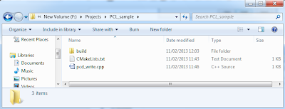
1. As shown in the following figure, create a folder for your project (here is PCL_sample). Within the folder, create one empty folder (for CMake output), a CMake config file (CMakeLists.txt) and entry of your project (pcd_write.cpp). An example of content of "CMakeLists.txt" and "pcd_write.cpp" can be found here.

Before CMake the project

2. Open the CMake and choose the directory for the source code and where to build the binaries, then click Configure.

Choose directory in CMake

3. In the pop-up window, choose the Visual Studio 10 (if your are using 64bit please select the corresponding one) and then click finish.

Pop-up window

4. After the build is finished, click the Generate button and you will see the VS2010 solution files are created in the build folder.

Finish build in CMake

VS 2010 solution file is created by the CMake

• Result

After compiling and running the program in VS2010, a point cloud data file (test_pcd.pcd in figure) is created. The basic data type is PointCloud which can be saved in *.pcd file by following format:

# .PCD v0.7 - Point Cloud Data file format
VERSION 0.7
FIELDS x y z
SIZE 4 4 4
TYPE F F F
COUNT 1 1 1
WIDTH 5
HEIGHT 1
VIEWPOINT 0 0 0 1 0 0 0
POINTS 5
DATA ascii
1.28125 577.09375 197.9375
828.125 599.03125 491.375
358.6875 917.4375 842.5625
764.5 178.28125 879.53125
727.53125 525.84375 311.28125

Output of pcd_write.cpp